I don’t know how I could miss this https://mathformeremortals.wordpress.com/ interesting blog. It stayed out of my radar until last week.
I strongly recommend the following posts, that I’ll keep ‘shortened’ here, just if the originals pass away in the future (beeing a wp blog is hard to conceive, but… who knows):
 With this mapping scheme we know that…
1 and 2 are adjacent.
2 and 3 are adjacent.
3 and 4 are adjacent.
4 and 5 are adjacent.
5 and 6 are NOT adjacent.
6 and 7 are adjacent…
If we look at coordinates along the y direction we also know that…
1 and 6 are adjacent.
2 and 7 are adjacent…
6 and 11 are adjacent…
In the 2D case the adjacencies were located along a number line. Everything was adjacent to its neighbors. In the 3D case the adjacencies are a little more complicated, but now that we know them, we can set up the bilinear interpolation and the derivatives.
With this mapping scheme we know that…
1 and 2 are adjacent.
2 and 3 are adjacent.
3 and 4 are adjacent.
4 and 5 are adjacent.
5 and 6 are NOT adjacent.
6 and 7 are adjacent…
If we look at coordinates along the y direction we also know that…
1 and 6 are adjacent.
2 and 7 are adjacent…
6 and 11 are adjacent…
In the 2D case the adjacencies were located along a number line. Everything was adjacent to its neighbors. In the 3D case the adjacencies are a little more complicated, but now that we know them, we can set up the bilinear interpolation and the derivatives.
 Calculate these proximities along both axes so that you can relate the input point’s position to these four nearby points on the output grid. The point’s weight with respect to the four nearby points is the product of its relative proximities in x and y, which is what we’re after. In the example J is the closest, so it has a weight of 51%. M is the furthest, so it only gets 6% of the weight.
 We are weighting the points using a linear measure even though we know we are working with a curved surface in 3D. That means this is only an approximation. The weighting works perfectly on a plane, and we are making the assumption that our surface will be locally planar. Even with a fairly coarse grid, this approximation works surprisingly well.
 If we’re using triangle interpolation, we need to choose a triangle that encloses the input point. If that triangle is JKL, then 50% of the weight goes to K and 50% goes to L. This is shown on the left side of the diagram in green. On the other hand, we can describe the same input point using triangle JKM shown on the right in orange. In that case the weight is shared between J and M. So which is it? KL or JM? On a 3D curved surface (which this probably is), these ostensibly equivalent schemes will yield different results.
Another case is where the input point is barely inside of the triangle like in this diagram shown in yellow. With triangle interpolation it is clear that JKL is the best triangle to use. However, almost all of the weight goes to K and L. What about Point J? (Or M?) The input point is nearly equidistant to these outer points, but the weight would not be distributed that way.
If we’re using triangle interpolation, we need to choose a triangle that encloses the input point. If that triangle is JKL, then 50% of the weight goes to K and 50% goes to L. This is shown on the left side of the diagram in green. On the other hand, we can describe the same input point using triangle JKM shown on the right in orange. In that case the weight is shared between J and M. So which is it? KL or JM? On a 3D curved surface (which this probably is), these ostensibly equivalent schemes will yield different results.
Another case is where the input point is barely inside of the triangle like in this diagram shown in yellow. With triangle interpolation it is clear that JKL is the best triangle to use. However, almost all of the weight goes to K and L. What about Point J? (Or M?) The input point is nearly equidistant to these outer points, but the weight would not be distributed that way.
 The bilinear approach (i.e. with four points) is the best approach for this kind of problem because the fourth point acts like a tie-breaker and avoids these ambiguities.
 In practice the input points may lie directly over or precisely between points in the output grid. When that happens, the weights in x or y (or both) take on values of 0 or 1 and there are less than four nonzero numbers in the equality condition. In this example rows 5 and 7 have more than 1 nonzero value. For example, Row 5 corresponds to the coordinate (2.5, 1), which is halfway between (2, 1) and (3, 1). For that reason Columns 8 and 9 share 50% of the weight for that point.
Using the sign conventions we used when we were regularizing 2D data, we call these Afidelity and bFidelity. Note that the equation is Az=b, not Ay=b like in the 2D case, because the output values are on the z axis instead of the y axis.
In practice the input points may lie directly over or precisely between points in the output grid. When that happens, the weights in x or y (or both) take on values of 0 or 1 and there are less than four nonzero numbers in the equality condition. In this example rows 5 and 7 have more than 1 nonzero value. For example, Row 5 corresponds to the coordinate (2.5, 1), which is halfway between (2, 1) and (3, 1). For that reason Columns 8 and 9 share 50% of the weight for that point.
Using the sign conventions we used when we were regularizing 2D data, we call these Afidelity and bFidelity. Note that the equation is Az=b, not Ay=b like in the 2D case, because the output values are on the z axis instead of the y axis.
 These interpolation numbers comprise the fidelity equations. The next step is to set up the second derivatives.
 In practice the input points may lie directly over or precisely between points in the output grid. When that happens, the weights in x or y (or both) take on values of 0 or 1 and there are fewer than four nonzero numbers in the equality condition. In this example rows 5 and 7 have more than 1 nonzero value. For example, Row 5 corresponds to the coordinate (2.5, 1), which is halfway between (2, 1) and (3, 1). For that reason Columns 8 and 9 share 50% of the weight for that point.
Using the sign conventions we used when we were regularizing 2D data, we call these AFidelity and bFidelity. Note that the equation is Az=b, not Ay=b like in the 2D case, because the output values are on the z axis instead of the y axis.
In practice the input points may lie directly over or precisely between points in the output grid. When that happens, the weights in x or y (or both) take on values of 0 or 1 and there are fewer than four nonzero numbers in the equality condition. In this example rows 5 and 7 have more than 1 nonzero value. For example, Row 5 corresponds to the coordinate (2.5, 1), which is halfway between (2, 1) and (3, 1). For that reason Columns 8 and 9 share 50% of the weight for that point.
Using the sign conventions we used when we were regularizing 2D data, we call these AFidelity and bFidelity. Note that the equation is Az=b, not Ay=b like in the 2D case, because the output values are on the z axis instead of the y axis.
 These interpolation numbers comprise the fidelity equations. The next step is to set up the second derivatives.
 The vertical derivatives have similar properties, but they show up at different locations in the matrix. Columns 1-5 have only one nonzero value (the value 1). Columns 6-10 have two nonzero values (1 and -2). Columns 11-15 have three nonzero values (1, -2, and 1 again). Then Columns 16-20 go back to two nonzero values and finally Columns 21-25 have only one nonzero value in them. This represents the way the vertical derivatives reuse rows in the output grid. There are five rows but only three ways to take second derivatives between those rows.
This Tetris-like animation shows how the vertical derivatives stack up based on the way the matrix columns map to points in the output grid. The center (representing the middle row of the output grid) has the highest stack of nonzero values because three derivative coefficients overlap there.
The vertical derivatives have similar properties, but they show up at different locations in the matrix. Columns 1-5 have only one nonzero value (the value 1). Columns 6-10 have two nonzero values (1 and -2). Columns 11-15 have three nonzero values (1, -2, and 1 again). Then Columns 16-20 go back to two nonzero values and finally Columns 21-25 have only one nonzero value in them. This represents the way the vertical derivatives reuse rows in the output grid. There are five rows but only three ways to take second derivatives between those rows.
This Tetris-like animation shows how the vertical derivatives stack up based on the way the matrix columns map to points in the output grid. The center (representing the middle row of the output grid) has the highest stack of nonzero values because three derivative coefficients overlap there.
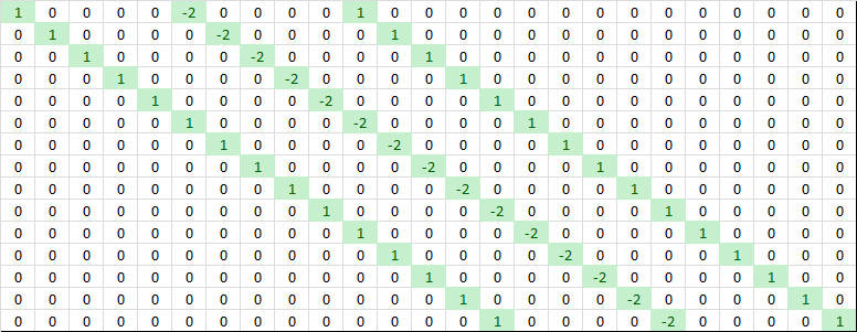 The two sets of derivatives have some interesting properties that are consistent with their role in this calculation process, and we can see these properties in the matrices visually. These details are not essential to know, but they are a good excuse to make a reference to Tetris!
 The only real difference is that there are more derivative equations because of the two directions x and y. If the output grid has the size MxN, then the number of derivative equations is related to that size. For example, a 25×4 grid has 142 derivative equations because there are 23 second derivatives to take within each column and there are 4 columns. There are 2 second derivatives that you can take in each row with 25 rows. That gives a total of 23 * 4 + 2 * 25 = 142. A 10×10 grid needs 80 + 80 = 160 derivative equations.
 In this example we have 7 input points (fidelity equations) and a 5×5 output grid, which gives us 30 second derivatives. Plugging those numbers into the equations with a smoothness constant KSmoothness of 0.5, we get…
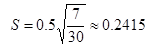 If we put it all together, we get this matrix A and vector b.
 At this point we have the overdetermined matrix equation with fidelity equations and scaled derivative equations. We can solve all of this for the least-squares solution z.
Download the Excel Spreadsheet – Data Regularization Examples in 3D
- https://mathformeremortals.wordpress.com/2013/07/22/introduction-to-regularizing-3d-data-part-1-of-2/
- https://mathformeremortals.wordpress.com/2013/07/24/introduction-to-regularizing-3d-data-part-2-of-2/
- https://mathformeremortals.wordpress.com/2014/04/05/minimize-and-minimizenonnegative-spreadsheet-optimization-v6/
How to Regularize 3D Data
Here is shown how to set up a 2D interpolation, and explains the difference between triangle interpolation and bilinear interpolation. It also shows how to set up the second derivatives for 3D data.
Working in 3D: Using a Grid Instead of a Number Line
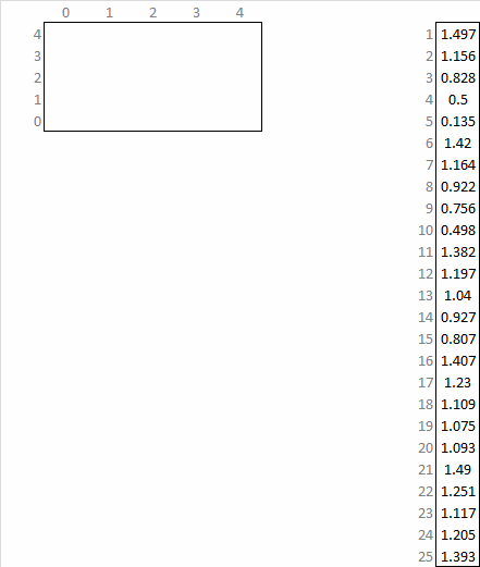
In the 2D case we mapped each input point to the corresponding one or two output points on a number line. In the 3D case the output points exist on a grid, so the number line concept won’t work. The tricky thing is that the output points still need to correspond to columns of a matrix, so they still have to be laid out in a straight line somehow. The way to solve this is to just pick matrix columns and assign them to points on the grid. This example uses a 5×5 grid, so we know there will be 25 distinct points on the output grid. That means we need a matrix with 25 columns, so let’s number those columns 1 – 25 and assign each grid point to a matrix column. There is no magic to it; any grid point can go with any matrix column as long as everything else is consistent with that. An intuitive way to map them is to group them by row and to number them in ascending order: 1-5, 6-10, 11-15, etc. The diagram below shows how the 25 output points are arranged on a grid, as does the animation at the beginning of this article.
With this mapping scheme we know that…
1 and 2 are adjacent.
2 and 3 are adjacent.
3 and 4 are adjacent.
4 and 5 are adjacent.
5 and 6 are NOT adjacent.
6 and 7 are adjacent…
If we look at coordinates along the y direction we also know that…
1 and 6 are adjacent.
2 and 7 are adjacent…
6 and 11 are adjacent…
In the 2D case the adjacencies were located along a number line. Everything was adjacent to its neighbors. In the 3D case the adjacencies are a little more complicated, but now that we know them, we can set up the bilinear interpolation and the derivatives.
Bilinear Interpolation
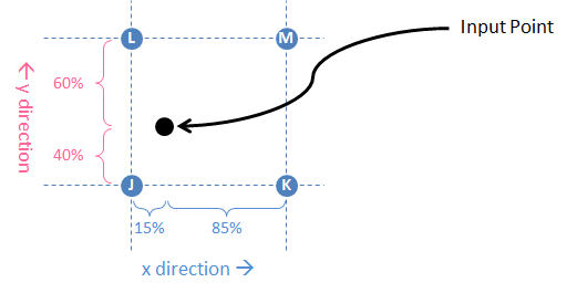
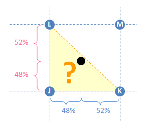
The bilinear interpolation equations are similar to the linear interpolation we did before. The first step is to identify the four output grid points that surround the input point. Those four points are labeled J, K, L, and M in the figure below. J, K, L, and M are not numerical values; they just identify the four points and, most importantly, their column numbers (1 – 25 in this example) in the matrix. Next we determine how far away those four points are to the input point in the X and Y directions separately. Those distances are measured as percentages of the total distance in each direction. For example, in the Y direction the input point is closest to J and K (40% of the Y distance) and further from L and M (60% of the Y distance). However, we swap these percentages and assign 60% to J and K and assign 40% to L and M. This works because we want to measure (and weight by) the “closeness” or “relative proximity” to the grid point, not the distance. A higher percentage indicates closer proximity (and therefore greater importance) and a lower percentage indicates less proximity.
Calculate these proximities along both axes so that you can relate the input point’s position to these four nearby points on the output grid. The point’s weight with respect to the four nearby points is the product of its relative proximities in x and y, which is what we’re after. In the example J is the closest, so it has a weight of 51%. M is the furthest, so it only gets 6% of the weight.
We are weighting the points using a linear measure even though we know we are working with a curved surface in 3D. That means this is only an approximation. The weighting works perfectly on a plane, and we are making the assumption that our surface will be locally planar. Even with a fairly coarse grid, this approximation works surprisingly well.
Why use four points? Can’t we do the same thing with three nearby points (i.e. triangle interpolation)?
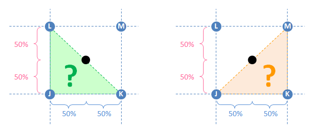
The answer is: Yes, but… Using four points is a more balanced approach because there are some inconsistencies with using only three points. For example, consider an input point like the one below – located exactly halfway between the four surrounding points JKLM.
If we’re using triangle interpolation, we need to choose a triangle that encloses the input point. If that triangle is JKL, then 50% of the weight goes to K and 50% goes to L. This is shown on the left side of the diagram in green. On the other hand, we can describe the same input point using triangle JKM shown on the right in orange. In that case the weight is shared between J and M. So which is it? KL or JM? On a 3D curved surface (which this probably is), these ostensibly equivalent schemes will yield different results.
Another case is where the input point is barely inside of the triangle like in this diagram shown in yellow. With triangle interpolation it is clear that JKL is the best triangle to use. However, almost all of the weight goes to K and L. What about Point J? (Or M?) The input point is nearly equidistant to these outer points, but the weight would not be distributed that way.
The bilinear approach (i.e. with four points) is the best approach for this kind of problem because the fourth point acts like a tie-breaker and avoids these ambiguities.
Implementing Bilinear Interpolation in the Spreadsheet
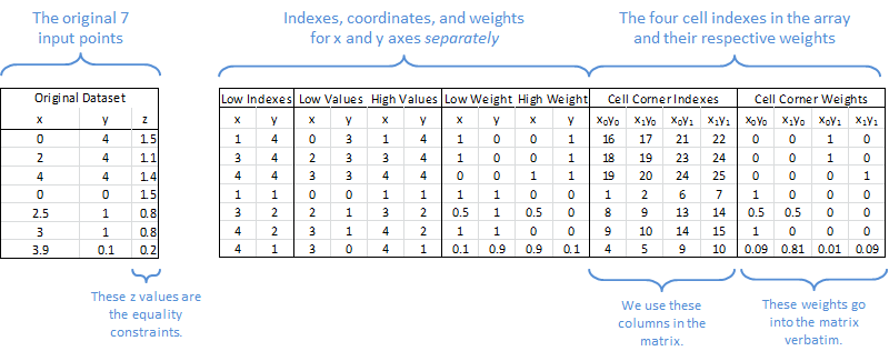
We want to map the x and y values onto the output grid (and thereby map them to those four points’ matrix columns) so that we can use the z values as equality constraints. In the spreadsheet the bilinear interpolation looks like this. The input points on the left are listed as seven x, y, and z values.
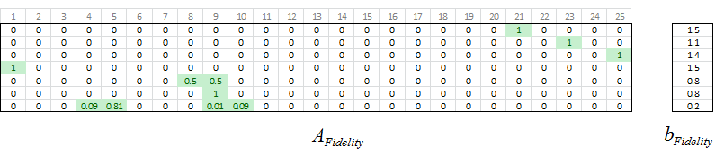
In practice the input points may lie directly over or precisely between points in the output grid. When that happens, the weights in x or y (or both) take on values of 0 or 1 and there are less than four nonzero numbers in the equality condition. In this example rows 5 and 7 have more than 1 nonzero value. For example, Row 5 corresponds to the coordinate (2.5, 1), which is halfway between (2, 1) and (3, 1). For that reason Columns 8 and 9 share 50% of the weight for that point.
Using the sign conventions we used when we were regularizing 2D data, we call these Afidelity and bFidelity. Note that the equation is Az=b, not Ay=b like in the 2D case, because the output values are on the z axis instead of the y axis.
These interpolation numbers comprise the fidelity equations. The next step is to set up the second derivatives.
An Entire 3D Surface from a Few Measured Points
- An investment banker needs to create an entire volatility surface from a handful of derivatives trades that took place today.
- A chemist needs to know the temperature near the center of a reaction chamber based on only a few temperature measurements scattered around its perimeter.
- An engineer needs to model something with a smooth function of two variables, but he doesn’t know the function and all he has are a few dozen noisy measurement points.
Implementing Bilinear Interpolation in the Spreadsheet
In the spreadsheet the bilinear interpolation looks like this. The input points on the left are listed as seven x, y, and z values. On the right are the logistics for bilinear interpolation.
In practice the input points may lie directly over or precisely between points in the output grid. When that happens, the weights in x or y (or both) take on values of 0 or 1 and there are fewer than four nonzero numbers in the equality condition. In this example rows 5 and 7 have more than 1 nonzero value. For example, Row 5 corresponds to the coordinate (2.5, 1), which is halfway between (2, 1) and (3, 1). For that reason Columns 8 and 9 share 50% of the weight for that point.
Using the sign conventions we used when we were regularizing 2D data, we call these AFidelity and bFidelity. Note that the equation is Az=b, not Ay=b like in the 2D case, because the output values are on the z axis instead of the y axis.
These interpolation numbers comprise the fidelity equations. The next step is to set up the second derivatives.
Second Derivatives – Vertical and Horizontal
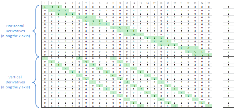
The second derivatives are calculated the same way as the 2D case, except that they are calculated separately for both axes, x and y. Just by looking at the diagram you can see that the horizontal derivatives are arranged in five clusters of three derivatives. With five adjacent points in our 5×5 output grid there are only three places where you can take a discrete second derivative, so each row in the output grid has three second derivatives. For example, Columns 1-5 are five columns, yet between those five columns there are only three second derivatives. The fourth second derivative begins in Column 6.
The vertical derivatives have similar properties, but they show up at different locations in the matrix. Columns 1-5 have only one nonzero value (the value 1). Columns 6-10 have two nonzero values (1 and -2). Columns 11-15 have three nonzero values (1, -2, and 1 again). Then Columns 16-20 go back to two nonzero values and finally Columns 21-25 have only one nonzero value in them. This represents the way the vertical derivatives reuse rows in the output grid. There are five rows but only three ways to take second derivatives between those rows.
This Tetris-like animation shows how the vertical derivatives stack up based on the way the matrix columns map to points in the output grid. The center (representing the middle row of the output grid) has the highest stack of nonzero values because three derivative coefficients overlap there.
The two sets of derivatives have some interesting properties that are consistent with their role in this calculation process, and we can see these properties in the matrices visually. These details are not essential to know, but they are a good excuse to make a reference to Tetris!
Smoothness Constant for 3D
In the 2D case the smoothness constant KSmoothness and the numbers of derivative and fidelity equations determine the derivative scaling factor S. As before, to give equal importance to smoothness and fitting, use KSmoothness = 1 (resulting in noticeable smoothing). If you want to give high importance to fitting your input points (as in 100 times as important), use KSmoothness = 0.01. If you want the result to be planar, use a high number like 5,000. S is derived from the sum of squared errors just like in the 2D case. For that reason it uses exactly the same equations.
The only real difference is that there are more derivative equations because of the two directions x and y. If the output grid has the size MxN, then the number of derivative equations is related to that size. For example, a 25×4 grid has 142 derivative equations because there are 23 second derivatives to take within each column and there are 4 columns. There are 2 second derivatives that you can take in each row with 25 rows. That gives a total of 23 * 4 + 2 * 25 = 142. A 10×10 grid needs 80 + 80 = 160 derivative equations.
If we put it all together, we get this matrix A and vector b.
At this point we have the overdetermined matrix equation with fidelity equations and scaled derivative equations. We can solve all of this for the least-squares solution z.
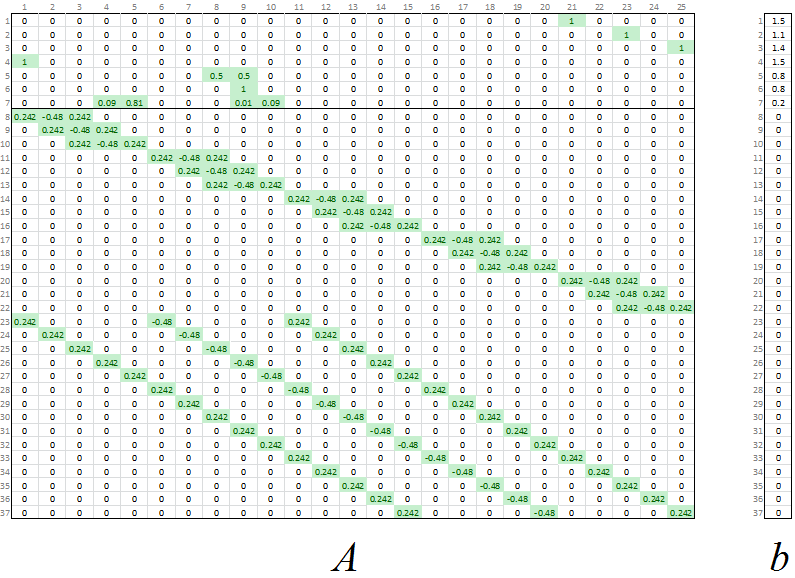
Normal Equations
As in the 2D case, we use the transpose of A to give the normal equations: (ATA)z = ATb. At this point it is just a matter of solving for z and mapping the result to the output grid.
Solution to the Normal Equations
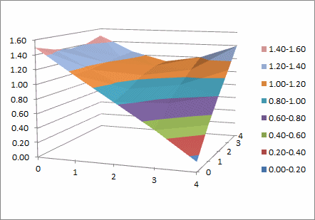
The solution is the vector of z values that satisfy the normal equations. Of course we need these numbers on a grid of x and y values so that the data are in 3D, so we map each z value to its location in the output grid. This animation shows how the 25×1 least-squares solution for z maps to our 5×5 output grid.
Download the Excel Spreadsheet – Data Regularization Examples in 3D